Loading And Visualizing mrr datA (LAVA)#

Acknowledgments should be given to Bobby Jackson and Zach Sherman for their help as well

Overview#

Within this notebook, we will cover:

General overview of the MRR and its variables
Reading the MRR data through the CROCUS Thredds Server
Visualizing the radar data

Prerequisites#

Concepts	Importance	Notes
Matplotlib Basics	Helpful	Basic plotting
NumPy Basics	Helpful	Basic arrays
Intro to Xarray	Helpful	Basic features

Time to learn: 45 minutes

Installation#

This is all the installation required to run this code.

conda env create -f mrr.yml

An Overview of the MRR-Pro#

The MRR-Pro is a vertically pointing weather radar located at Northeastern Illinois University used to measure rain. It is used to collect data like reflectivity, radial velocity, drop size distribution, log attenuated power, signal to noise ratio, melting layer, doppler spectrum width, rainfall rate, and liquid water content.

Imports#

import numpy as np
import matplotlib.pyplot as plt
from matplotlib.dates import DateFormatter
import warnings
warnings.filterwarnings("ignore")
from siphon.catalog import TDSCatalog
import xarray as xr
import sys
import cmweather

Data Preprocessing#

Define a function used to make sure no files without data are counted.

def catch_bad_file(cds):
    try:
        return cds.remote_access(use_xarray=True)
    except:
        print("Exception: ", sys.exc_info()[0])

Accessing the CROCUS Thredds server#

The TDSCatalog is an object that stores the description of the THREDDS server. In this case it takes the CROCUS Thredds server URL. This creates a catalog of all the files so it is easier to call and use them.

cat_url = 'https://thredds.crocus-urban.org/thredds/catalog/neiu-mrrpro-a1/catalog.html'
cat = TDSCatalog(cat_url)
print(list(cat.datasets.keys()))

---------------------------------------------------------------------------
HTTPError                                 Traceback (most recent call last)
Cell In[3], line 2
      1 cat_url = 'https://thredds.crocus-urban.org/thredds/catalog/neiu-mrrpro-a1/catalog.html'
----> 2 cat = TDSCatalog(cat_url)
      3 print(list(cat.datasets.keys()))

File ~/miniconda3/envs/instrument-cookbooks-dev/lib/python3.10/site-packages/siphon/catalog.py:289, in TDSCatalog.__init__(self, catalog_url)
    287 # get catalog.xml file
    288 resp = self.session.get(catalog_url)
--> 289 resp.raise_for_status()
    291 # top level server url
    292 self.catalog_url = resp.url

File ~/miniconda3/envs/instrument-cookbooks-dev/lib/python3.10/site-packages/requests/models.py:1024, in Response.raise_for_status(self)
   1019     http_error_msg = (
   1020         f"{self.status_code} Server Error: {reason} for url: {self.url}"
   1021     )
   1023 if http_error_msg:
-> 1024     raise HTTPError(http_error_msg, response=self)

HTTPError: 502 Server Error: Bad Gateway for url: https://thredds.crocus-urban.org/thredds/catalog/neiu-mrrpro-a1/catalog.html

Testing the code#

Let’s do a test to see if you are able to access files on the Thredds server and if all the correct packages are installed. We will start with 2 files for now and will have to adjust for the time frames later. Eventually if you wanted to use the whole catalog you just need to change, for cds in cat.datasets[1:3]

dsets = [catch_bad_file(cds)
         for cds in cat.datasets[1:3]]
# removes empty datasets
ds_non_none = [x for x in dsets if x is not None]
ds = xr.combine_by_coords(ds_non_none, combine_attrs='override')

Shows the variables and names of the data in the dataset that can be used.

dsets

[<xarray.Dataset>
 Dimensions:                 (range: 256, sweep: 1, time: 360, n_spectra: 256,
                              spectrum_n_samples: 32)
 Coordinates:
   * range                   (range) float32 0.0 35.0 70.0 ... 8.89e+03 8.925e+03
   * time                    (time) datetime64[ns] 2023-06-01T02:00:00.0011051...
     elevation               (time) float32 ...
     azimuth                 (time) float32 ...
 Dimensions without coordinates: sweep, n_spectra, spectrum_n_samples
 Data variables: (12/31)
     volume_number           int32 ...
     time_coverage_start     |S128 ...
     time_coverage_end       |S128 ...
     time_reference          |S128 ...
     instrument_type         |S128 ...
     transfer_function       (range) float64 ...
     ...                      ...
     ML                      (time, range) float64 ...
     SNR                     (time, range) float32 ...
     index_spectra           (time, range) float64 ...
     spectrum_raw            (time, n_spectra, spectrum_n_samples) float64 ...
     N                       (time, n_spectra, spectrum_n_samples) float64 ...
     D                       (n_spectra, spectrum_n_samples) float64 ...
 Attributes:
     Conventions:      CF/Radial
     version:          1.3
     title:            METEK MRR Pro 1.2.5 Data
     institution:      None
     references:       None
     source:           None
     history:          None
     comment:          None
     instrument_name:  METEK MRR Pro 1.2.5, ID: MRRPro97, METEK Serial Number:...
     site_name:        cms-mrr-002
     field_names:      Za,Z,Zea,Ze,RR,LWC,PIA,VEL,WIDTH,SNR,spectrum_reflectiv...,
 <xarray.Dataset>
 Dimensions:                 (range: 256, sweep: 1, time: 360, n_spectra: 256,
                              spectrum_n_samples: 32)
 Coordinates:
   * range                   (range) float32 0.0 35.0 70.0 ... 8.89e+03 8.925e+03
   * time                    (time) datetime64[ns] 2023-06-01T04:00:00.0010859...
     elevation               (time) float32 ...
     azimuth                 (time) float32 ...
 Dimensions without coordinates: sweep, n_spectra, spectrum_n_samples
 Data variables: (12/31)
     volume_number           int32 ...
     time_coverage_start     |S128 ...
     time_coverage_end       |S128 ...
     time_reference          |S128 ...
     instrument_type         |S128 ...
     transfer_function       (range) float64 ...
     ...                      ...
     ML                      (time, range) float64 ...
     SNR                     (time, range) float32 ...
     index_spectra           (time, range) float64 ...
     spectrum_raw            (time, n_spectra, spectrum_n_samples) float64 ...
     N                       (time, n_spectra, spectrum_n_samples) float64 ...
     D                       (n_spectra, spectrum_n_samples) float64 ...
 Attributes:
     Conventions:      CF/Radial
     version:          1.3
     title:            METEK MRR Pro 1.2.5 Data
     institution:      None
     references:       None
     source:           None
     history:          None
     comment:          None
     instrument_name:  METEK MRR Pro 1.2.5, ID: MRRPro97, METEK Serial Number:...
     site_name:        cms-mrr-002
     field_names:      Za,Z,Zea,Ze,RR,LWC,PIA,VEL,WIDTH,SNR,spectrum_reflectiv...]

Shows the times that are being plotted.

ds['Ze']

<xarray.DataArray 'Ze' (time: 720, range: 256)>
array([[nan, nan, nan, ..., nan, nan, nan],
       [nan, nan, nan, ..., nan, nan, nan],
       [nan, nan, nan, ..., nan, nan, nan],
       ...,
       [nan, nan, nan, ..., nan, nan, nan],
       [nan, nan, nan, ..., nan, nan, nan],
       [nan, nan, nan, ..., nan, nan, nan]])
Coordinates:
  * range      (range) float32 0.0 35.0 70.0 ... 8.855e+03 8.89e+03 8.925e+03
  * time       (time) datetime64[ns] 2023-06-01T02:00:00.001105152 ... 2023-0...
    elevation  (time) float32 90.0 90.0 90.0 90.0 90.0 ... 90.0 90.0 90.0 90.0
    azimuth    (time) float32 0.0 0.0 0.0 0.0 0.0 0.0 ... 0.0 0.0 0.0 0.0 0.0
Attributes:
    standard_name:     equivalent_reflectivity_factor
    long_name:         None
    units:             dBZ
    field_folds:       false
    fold_limit_lower:  0.0
    fold_limit_upper:  0.0
    thresholding_xml:  None
    legend_xml:        None
    is_discreet:       false
    _ChunkSizes:       [  1 256]

xarray.DataArray

'Ze'

time: 720
range: 256

nan nan nan nan nan nan nan nan ... nan nan nan nan nan nan nan nan

array([[nan, nan, nan, ..., nan, nan, nan],
       [nan, nan, nan, ..., nan, nan, nan],
       [nan, nan, nan, ..., nan, nan, nan],
       ...,
       [nan, nan, nan, ..., nan, nan, nan],
       [nan, nan, nan, ..., nan, nan, nan],
       [nan, nan, nan, ..., nan, nan, nan]])

Coordinates: (4)

range
(range)
float32
0.0 35.0 ... 8.89e+03 8.925e+03
standard_name :
projection_range_coordinate
long_name :
range_to_measurement_volume
units :
meters
spacing_is_constant :
true
meters_to_center_of_first_gate :
0.0
meters_between_gates :
35.0
axis :
radial_range_coordinate
```
array([   0.,   35.,   70., ..., 8855., 8890., 8925.], dtype=float32)
```

time

(time)

datetime64[ns]

2023-06-01T02:00:00.001105152 .....

long_name :: time_in_seconds_since_volume_start
standard_name :: time
_ChunkSizes :: 512

array(['2023-06-01T02:00:00.001105152', '2023-06-01T02:00:10.001099008',
       '2023-06-01T02:00:20.001112064', ..., '2023-06-01T04:59:30.001105152',
       '2023-06-01T04:59:40.001081088', '2023-06-01T04:59:50.001081088'],
      dtype='datetime64[ns]')

elevation

(time)

float32

90.0 90.0 90.0 ... 90.0 90.0 90.0

standard_name :: ray_elevation_angle
long_name :: elevation_angle_from_horizontal_plane
units :: degrees
axis :: radial_elevation_coordinate
_ChunkSizes :: 1024

array([90., 90., 90., 90., 90., 90., 90., 90., 90., 90., 90., 90., 90.,
       90., 90., 90., 90., 90., 90., 90., 90., 90., 90., 90., 90., 90.,
       90., 90., 90., 90., 90., 90., 90., 90., 90., 90., 90., 90., 90.,
       90., 90., 90., 90., 90., 90., 90., 90., 90., 90., 90., 90., 90.,
       90., 90., 90., 90., 90., 90., 90., 90., 90., 90., 90., 90., 90.,
       90., 90., 90., 90., 90., 90., 90., 90., 90., 90., 90., 90., 90.,
       90., 90., 90., 90., 90., 90., 90., 90., 90., 90., 90., 90., 90.,
       90., 90., 90., 90., 90., 90., 90., 90., 90., 90., 90., 90., 90.,
       90., 90., 90., 90., 90., 90., 90., 90., 90., 90., 90., 90., 90.,
       90., 90., 90., 90., 90., 90., 90., 90., 90., 90., 90., 90., 90.,
       90., 90., 90., 90., 90., 90., 90., 90., 90., 90., 90., 90., 90.,
       90., 90., 90., 90., 90., 90., 90., 90., 90., 90., 90., 90., 90.,
       90., 90., 90., 90., 90., 90., 90., 90., 90., 90., 90., 90., 90.,
       90., 90., 90., 90., 90., 90., 90., 90., 90., 90., 90., 90., 90.,
       90., 90., 90., 90., 90., 90., 90., 90., 90., 90., 90., 90., 90.,
       90., 90., 90., 90., 90., 90., 90., 90., 90., 90., 90., 90., 90.,
       90., 90., 90., 90., 90., 90., 90., 90., 90., 90., 90., 90., 90.,
       90., 90., 90., 90., 90., 90., 90., 90., 90., 90., 90., 90., 90.,
       90., 90., 90., 90., 90., 90., 90., 90., 90., 90., 90., 90., 90.,
       90., 90., 90., 90., 90., 90., 90., 90., 90., 90., 90., 90., 90.,
...
       90., 90., 90., 90., 90., 90., 90., 90., 90., 90., 90., 90., 90.,
       90., 90., 90., 90., 90., 90., 90., 90., 90., 90., 90., 90., 90.,
       90., 90., 90., 90., 90., 90., 90., 90., 90., 90., 90., 90., 90.,
       90., 90., 90., 90., 90., 90., 90., 90., 90., 90., 90., 90., 90.,
       90., 90., 90., 90., 90., 90., 90., 90., 90., 90., 90., 90., 90.,
       90., 90., 90., 90., 90., 90., 90., 90., 90., 90., 90., 90., 90.,
       90., 90., 90., 90., 90., 90., 90., 90., 90., 90., 90., 90., 90.,
       90., 90., 90., 90., 90., 90., 90., 90., 90., 90., 90., 90., 90.,
       90., 90., 90., 90., 90., 90., 90., 90., 90., 90., 90., 90., 90.,
       90., 90., 90., 90., 90., 90., 90., 90., 90., 90., 90., 90., 90.,
       90., 90., 90., 90., 90., 90., 90., 90., 90., 90., 90., 90., 90.,
       90., 90., 90., 90., 90., 90., 90., 90., 90., 90., 90., 90., 90.,
       90., 90., 90., 90., 90., 90., 90., 90., 90., 90., 90., 90., 90.,
       90., 90., 90., 90., 90., 90., 90., 90., 90., 90., 90., 90., 90.,
       90., 90., 90., 90., 90., 90., 90., 90., 90., 90., 90., 90., 90.,
       90., 90., 90., 90., 90., 90., 90., 90., 90., 90., 90., 90., 90.,
       90., 90., 90., 90., 90., 90., 90., 90., 90., 90., 90., 90., 90.,
       90., 90., 90., 90., 90., 90., 90., 90., 90., 90., 90., 90., 90.,
       90., 90., 90., 90., 90., 90., 90., 90., 90., 90., 90., 90., 90.,
       90., 90., 90., 90., 90.], dtype=float32)

azimuth

(time)

float32

0.0 0.0 0.0 0.0 ... 0.0 0.0 0.0 0.0

standard_name :: ray_azimuth_angle
long_name :: azimuth_angle_from_true_north
units :: degrees
axis :: radial_azimuth_coordinate
_ChunkSizes :: 1024

array([0., 0., 0., 0., 0., 0., 0., 0., 0., 0., 0., 0., 0., 0., 0., 0., 0.,
       0., 0., 0., 0., 0., 0., 0., 0., 0., 0., 0., 0., 0., 0., 0., 0., 0.,
       0., 0., 0., 0., 0., 0., 0., 0., 0., 0., 0., 0., 0., 0., 0., 0., 0.,
       0., 0., 0., 0., 0., 0., 0., 0., 0., 0., 0., 0., 0., 0., 0., 0., 0.,
       0., 0., 0., 0., 0., 0., 0., 0., 0., 0., 0., 0., 0., 0., 0., 0., 0.,
       0., 0., 0., 0., 0., 0., 0., 0., 0., 0., 0., 0., 0., 0., 0., 0., 0.,
       0., 0., 0., 0., 0., 0., 0., 0., 0., 0., 0., 0., 0., 0., 0., 0., 0.,
       0., 0., 0., 0., 0., 0., 0., 0., 0., 0., 0., 0., 0., 0., 0., 0., 0.,
       0., 0., 0., 0., 0., 0., 0., 0., 0., 0., 0., 0., 0., 0., 0., 0., 0.,
       0., 0., 0., 0., 0., 0., 0., 0., 0., 0., 0., 0., 0., 0., 0., 0., 0.,
       0., 0., 0., 0., 0., 0., 0., 0., 0., 0., 0., 0., 0., 0., 0., 0., 0.,
       0., 0., 0., 0., 0., 0., 0., 0., 0., 0., 0., 0., 0., 0., 0., 0., 0.,
       0., 0., 0., 0., 0., 0., 0., 0., 0., 0., 0., 0., 0., 0., 0., 0., 0.,
       0., 0., 0., 0., 0., 0., 0., 0., 0., 0., 0., 0., 0., 0., 0., 0., 0.,
       0., 0., 0., 0., 0., 0., 0., 0., 0., 0., 0., 0., 0., 0., 0., 0., 0.,
       0., 0., 0., 0., 0., 0., 0., 0., 0., 0., 0., 0., 0., 0., 0., 0., 0.,
       0., 0., 0., 0., 0., 0., 0., 0., 0., 0., 0., 0., 0., 0., 0., 0., 0.,
       0., 0., 0., 0., 0., 0., 0., 0., 0., 0., 0., 0., 0., 0., 0., 0., 0.,
       0., 0., 0., 0., 0., 0., 0., 0., 0., 0., 0., 0., 0., 0., 0., 0., 0.,
       0., 0., 0., 0., 0., 0., 0., 0., 0., 0., 0., 0., 0., 0., 0., 0., 0.,
...
       0., 0., 0., 0., 0., 0., 0., 0., 0., 0., 0., 0., 0., 0., 0., 0., 0.,
       0., 0., 0., 0., 0., 0., 0., 0., 0., 0., 0., 0., 0., 0., 0., 0., 0.,
       0., 0., 0., 0., 0., 0., 0., 0., 0., 0., 0., 0., 0., 0., 0., 0., 0.,
       0., 0., 0., 0., 0., 0., 0., 0., 0., 0., 0., 0., 0., 0., 0., 0., 0.,
       0., 0., 0., 0., 0., 0., 0., 0., 0., 0., 0., 0., 0., 0., 0., 0., 0.,
       0., 0., 0., 0., 0., 0., 0., 0., 0., 0., 0., 0., 0., 0., 0., 0., 0.,
       0., 0., 0., 0., 0., 0., 0., 0., 0., 0., 0., 0., 0., 0., 0., 0., 0.,
       0., 0., 0., 0., 0., 0., 0., 0., 0., 0., 0., 0., 0., 0., 0., 0., 0.,
       0., 0., 0., 0., 0., 0., 0., 0., 0., 0., 0., 0., 0., 0., 0., 0., 0.,
       0., 0., 0., 0., 0., 0., 0., 0., 0., 0., 0., 0., 0., 0., 0., 0., 0.,
       0., 0., 0., 0., 0., 0., 0., 0., 0., 0., 0., 0., 0., 0., 0., 0., 0.,
       0., 0., 0., 0., 0., 0., 0., 0., 0., 0., 0., 0., 0., 0., 0., 0., 0.,
       0., 0., 0., 0., 0., 0., 0., 0., 0., 0., 0., 0., 0., 0., 0., 0., 0.,
       0., 0., 0., 0., 0., 0., 0., 0., 0., 0., 0., 0., 0., 0., 0., 0., 0.,
       0., 0., 0., 0., 0., 0., 0., 0., 0., 0., 0., 0., 0., 0., 0., 0., 0.,
       0., 0., 0., 0., 0., 0., 0., 0., 0., 0., 0., 0., 0., 0., 0., 0., 0.,
       0., 0., 0., 0., 0., 0., 0., 0., 0., 0., 0., 0., 0., 0., 0., 0., 0.,
       0., 0., 0., 0., 0., 0., 0., 0., 0., 0., 0., 0., 0., 0., 0., 0., 0.,
       0., 0., 0., 0., 0., 0., 0., 0., 0., 0., 0., 0., 0., 0., 0., 0., 0.,
       0., 0., 0., 0., 0., 0.], dtype=float32)

Indexes: (2)

range

PandasIndex

PandasIndex(Float64Index([   0.0,   35.0,   70.0,  105.0,  140.0,  175.0,  210.0,  245.0,
               280.0,  315.0,
              ...
              8610.0, 8645.0, 8680.0, 8715.0, 8750.0, 8785.0, 8820.0, 8855.0,
              8890.0, 8925.0],
             dtype='float64', name='range', length=256))

time

PandasIndex

PandasIndex(DatetimeIndex(['2023-06-01 02:00:00.001105152',
               '2023-06-01 02:00:10.001099008',
               '2023-06-01 02:00:20.001112064',
               '2023-06-01 02:00:30.001082880',
               '2023-06-01 02:00:40.001101056',
               '2023-06-01 02:00:50.001086976',
               '2023-06-01 02:01:00.001084928',
               '2023-06-01 02:01:10.001075968',
               '2023-06-01 02:01:20.001096960',
               '2023-06-01 02:01:30.001099008',
               ...
               '2023-06-01 04:58:20.001082880',
               '2023-06-01 04:58:30.001091072',
               '2023-06-01 04:58:40.001095936',
               '2023-06-01 04:58:50.001089024',
               '2023-06-01 04:59:00.001095936',
               '2023-06-01 04:59:10.001101056',
               '2023-06-01 04:59:20.001084928',
               '2023-06-01 04:59:30.001105152',
               '2023-06-01 04:59:40.001081088',
               '2023-06-01 04:59:50.001081088'],
              dtype='datetime64[ns]', name='time', length=720, freq=None))

Attributes: (10)
standard_name :
equivalent_reflectivity_factor
long_name :
None
units :
dBZ
field_folds :
false
fold_limit_lower :
0.0
fold_limit_upper :
0.0
thresholding_xml :
None
legend_xml :
None
is_discreet :
false
_ChunkSizes :
[ 1 256]

Sample plot using the test data#

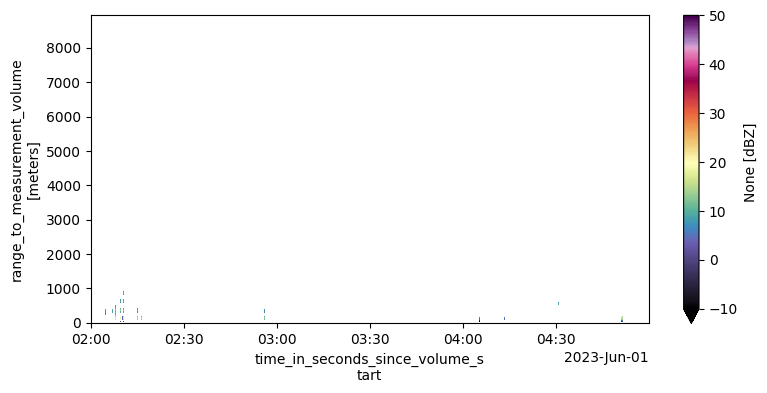
Plotting the figure and as you can see there is no precipitation.

plt.figure(figsize=(9, 4))
ds['Ze'].plot(x='time', cmap='ChaseSpectral', vmin=-10, vmax=50)
# Uncomment if you want to save and rename the figure
#plt.savefig('June 15.png', dpi=300, bbox_inches='tight')

<matplotlib.collections.QuadMesh at 0x14c4642e0>

../../_images/3009b73f74f81e24e698653b26756ad79b029ffc77ea3024dd9326c326614b0b.png

Visualizing the MRR data#

Plotting one hour in a single plot#

The code cell below picks one hour in a single day and downloads it as a dataset and displays its attributes.

ds = cat.datasets[297]
ds = ds.remote_access(use_xarray=True)
ds

<xarray.Dataset>
Dimensions:                 (range: 256, sweep: 1, time: 360, n_spectra: 256,
                             spectrum_n_samples: 32)
Coordinates:
  * range                   (range) float32 0.0 35.0 70.0 ... 8.89e+03 8.925e+03
  * time                    (time) datetime64[ns] 2023-07-15T19:00:00.0067289...
    elevation               (time) float32 ...
    azimuth                 (time) float32 ...
Dimensions without coordinates: sweep, n_spectra, spectrum_n_samples
Data variables: (12/31)
    volume_number           int32 ...
    time_coverage_start     |S128 ...
    time_coverage_end       |S128 ...
    time_reference          |S128 ...
    instrument_type         |S128 ...
    transfer_function       (range) float64 ...
    ...                      ...
    ML                      (time, range) float64 ...
    SNR                     (time, range) float32 ...
    index_spectra           (time, range) float64 ...
    spectrum_raw            (time, n_spectra, spectrum_n_samples) float64 ...
    N                       (time, n_spectra, spectrum_n_samples) float64 ...
    D                       (n_spectra, spectrum_n_samples) float64 ...
Attributes:
    Conventions:      CF/Radial
    version:          1.3
    title:            METEK MRR Pro 1.2.5 Data
    institution:      None
    references:       None
    source:           None
    history:          None
    comment:          None
    instrument_name:  METEK MRR Pro 1.2.5, ID: MRRPro97, METEK Serial Number:...
    site_name:        cms-mrr-002
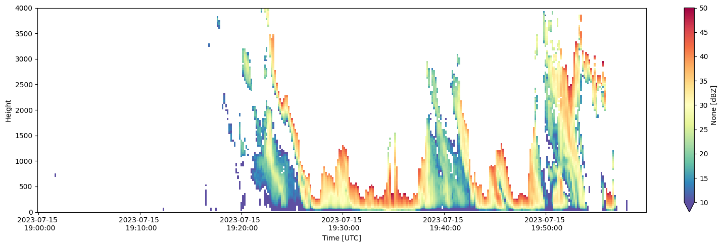
    field_names:      Za,Z,Zea,Ze,RR,LWC,PIA,VEL,WIDTH,SNR,spectrum_reflectiv...

xarray.Dataset

Dimensions:
- range: 256
- sweep: 1
- time: 360
- n_spectra: 256
- spectrum_n_samples: 32
Coordinates: (4)
- range
  (range)
  float32
  0.0 35.0 ... 8.89e+03 8.925e+03
  standard_name :
  projection_range_coordinate
  long_name :
  range_to_measurement_volume
  units :
  meters
  spacing_is_constant :
  true
  meters_to_center_of_first_gate :
  0.0
  meters_between_gates :
  35.0
  axis :
  radial_range_coordinate
```
array([   0.,   35.,   70., ..., 8855., 8890., 8925.], dtype=float32)
```
- time
  (time)
  datetime64[ns]
  2023-07-15T19:00:00.006728960 .....
  long_name :
  time_in_seconds_since_volume_start
  standard_name :
  time
  _ChunkSizes :
  512
```
array(['2023-07-15T19:00:00.006728960', '2023-07-15T19:00:10.006705920',
       '2023-07-15T19:00:20.006712832', ..., '2023-07-15T19:59:30.006707968',
       '2023-07-15T19:59:40.006707968', '2023-07-15T19:59:50.006724096'],
      dtype='datetime64[ns]')
```
- elevation
  (time)
  float32
  ...
  standard_name :
  ray_elevation_angle
  long_name :
  elevation_angle_from_horizontal_plane
  units :
  degrees
  axis :
  radial_elevation_coordinate
  _ChunkSizes :
  1024
```
[360 values with dtype=float32]
```
- azimuth
  (time)
  float32
  ...
  standard_name :
  ray_azimuth_angle
  long_name :
  azimuth_angle_from_true_north
  units :
  degrees
  axis :
  radial_azimuth_coordinate
  _ChunkSizes :
  1024
```
[360 values with dtype=float32]
```
Data variables: (31)
- volume_number
  ()
  int32
  ...
```
[1 values with dtype=int32]
```
- time_coverage_start
  ()
  |S128
  ...
```
[1 values with dtype=|S128]
```
- time_coverage_end
  ()
  |S128
  ...
```
[1 values with dtype=|S128]
```
- time_reference
  ()
  |S128
  ...
```
[1 values with dtype=|S128]
```
- instrument_type
  ()
  |S128
  ...
```
[1 values with dtype=|S128]
```
- transfer_function
  (range)
  float64
  ...
```
[256 values with dtype=float64]
```
- calibration_constant
  ()
  float64
  ...
```
[1 values with dtype=float64]
```
- latitude
  ()
  float64
  ...
  units :
  degrees_north
```
[1 values with dtype=float64]
```
- longitude
  ()
  float64
  ...
  units :
  degrees_east
```
[1 values with dtype=float64]
```
- altitude
  ()
  float64
  ...
  units :
  meters
```
[1 values with dtype=float64]
```
- doppler_shift_spectrum
  ()
  float64
  ...
```
[1 values with dtype=float64]
```
- sweep_number
  (sweep)
  int32
  ...
```
[1 values with dtype=int32]
```
- sweep_mode
  (sweep)
  |S128
  ...
```
[1 values with dtype=|S128]
```
- fixed_angle
  (sweep)
  float32
  ...
```
[1 values with dtype=float32]
```
- sweep_start_ray_index
  (sweep)
  int32
  ...
```
[1 values with dtype=int32]
```
- sweep_end_ray_index
  (sweep)
  int32
  ...
```
[1 values with dtype=int32]
```
- Za
  (time, range)
  float32
  ...
  standard_name :
  log_attenuated_reflectivity
  long_name :
  None
  units :
  dBZ
  field_folds :
  false
  fold_limit_lower :
  0.0
  fold_limit_upper :
  0.0
  thresholding_xml :
  None
  legend_xml :
  None
  is_discreet :
  false
  _ChunkSizes :
  [ 1 256]
```
[92160 values with dtype=float32]
```
- Z
  (time, range)
  float64
  ...
  standard_name :
  log_reflectivity
  long_name :
  None
  units :
  dBZ
  field_folds :
  false
  fold_limit_lower :
  0.0
  fold_limit_upper :
  0.0
  thresholding_xml :
  None
  legend_xml :
  None
  is_discreet :
  false
  _ChunkSizes :
  [ 1 256]
```
[92160 values with dtype=float64]
```
- Zea
  (time, range)
  float64
  ...
  standard_name :
  attenuated_equivalent_reflectivity_factor
  long_name :
  None
  units :
  dBZ
  field_folds :
  false
  fold_limit_lower :
  0.0
  fold_limit_upper :
  0.0
  thresholding_xml :
  None
  legend_xml :
  None
  is_discreet :
  false
  _ChunkSizes :
  [ 1 256]
```
[92160 values with dtype=float64]
```
- Ze
  (time, range)
  float64
  ...
  standard_name :
  equivalent_reflectivity_factor
  long_name :
  None
  units :
  dBZ
  field_folds :
  false
  fold_limit_lower :
  0.0
  fold_limit_upper :
  0.0
  thresholding_xml :
  None
  legend_xml :
  None
  is_discreet :
  false
  _ChunkSizes :
  [ 1 256]
```
[92160 values with dtype=float64]
```
- RR
  (time, range)
  float64
  ...
  standard_name :
  rainfall_rate
  long_name :
  None
  units :
  mm h-1
  field_folds :
  false
  fold_limit_lower :
  0.0
  fold_limit_upper :
  0.0
  thresholding_xml :
  None
  legend_xml :
  None
  is_discreet :
  false
  _ChunkSizes :
  [ 1 256]
```
[92160 values with dtype=float64]
```
- LWC
  (time, range)
  float64
  ...
  standard_name :
  mass_concentration_of_liquid_water_in_air
  long_name :
  None
  units :
  g m-3
  field_folds :
  false
  fold_limit_lower :
  0.0
  fold_limit_upper :
  0.0
  thresholding_xml :
  None
  legend_xml :
  None
  is_discreet :
  false
  _ChunkSizes :
  [ 1 256]
```
[92160 values with dtype=float64]
```
- PIA
  (time, range)
  float64
  ...
  standard_name :
  path_integrated_rain_attenuation
  long_name :
  None
  units :
  dB
  field_folds :
  false
  fold_limit_lower :
  0.0
  fold_limit_upper :
  0.0
  thresholding_xml :
  None
  legend_xml :
  None
  is_discreet :
  false
  _ChunkSizes :
  [ 1 256]
```
[92160 values with dtype=float64]
```
- VEL
  (time, range)
  float32
  ...
  standard_name :
  radial_velocity_of_scatterers_towards_instrument
  long_name :
  None
  units :
  m s-1
  field_folds :
  true
  fold_limit_lower :
  -0.0
  fold_limit_upper :
  5.8507977
  thresholding_xml :
  None
  legend_xml :
  None
  is_discreet :
  false
  _ChunkSizes :
  [ 1 256]
```
[92160 values with dtype=float32]
```
- WIDTH
  (time, range)
  float64
  ...
  standard_name :
  doppler_spectrum_width
  long_name :
  None
  units :
  m/s
  field_folds :
  false
  fold_limit_lower :
  0.0
  fold_limit_upper :
  0.0
  thresholding_xml :
  None
  legend_xml :
  None
  is_discreet :
  false
  _ChunkSizes :
  [ 1 256]
```
[92160 values with dtype=float64]
```
- ML
  (time, range)
  float64
  ...
  standard_name :
  melting_layer
  long_name :
  None
  units :
  None
  field_folds :
  false
  fold_limit_lower :
  0.0
  fold_limit_upper :
  0.0
  thresholding_xml :
  None
  legend_xml :
  None
  is_discreet :
  false
  _ChunkSizes :
  [ 1 256]
```
[92160 values with dtype=float64]
```
- SNR
  (time, range)
  float32
  ...
  standard_name :
  signal_to_noise_ratio
  long_name :
  None
  units :
  dB
  field_folds :
  false
  fold_limit_lower :
  0.0
  fold_limit_upper :
  0.0
  thresholding_xml :
  None
  legend_xml :
  None
  is_discreet :
  false
  _ChunkSizes :
  [ 1 256]
```
[92160 values with dtype=float32]
```
- index_spectra
  (time, range)
  float64
  ...
  standard_name :
  index variable spectra
  long_name :
  None
  units :
  None
  field_folds :
  false
  fold_limit_lower :
  0.0
  fold_limit_upper :
  0.0
  thresholding_xml :
  None
  legend_xml :
  None
  is_discreet :
  true
  _ChunkSizes :
  [ 1 256]
```
[92160 values with dtype=float64]
```
- spectrum_raw
  (time, n_spectra, spectrum_n_samples)
  float64
  ...
  standard_name :
  log_attenuated_power
  long_name :
  None
  units :
  dB
  index_var_name :
  None
  block_avg_length :
  0
  is_spectrum :
  true
  _ChunkSizes :
  [ 1 256 32]
```
[2949120 values with dtype=float64]
```
- N
  (time, n_spectra, spectrum_n_samples)
  float64
  ...
  standard_name :
  drop_size_distribution
  long_name :
  None
  units :
  1
  index_var_name :
  None
  block_avg_length :
  0
  is_spectrum :
  true
  _ChunkSizes :
  [ 1 256 32]
```
[2949120 values with dtype=float64]
```
- D
  (n_spectra, spectrum_n_samples)
  float64
  ...
  standard_name :
  drop_sizes
  long_name :
  None
  units :
  1
  index_var_name :
  None
  block_avg_length :
  0
  is_spectrum :
  true
```
[8192 values with dtype=float64]
```

Indexes: (2)

range

PandasIndex

PandasIndex(Float64Index([   0.0,   35.0,   70.0,  105.0,  140.0,  175.0,  210.0,  245.0,
               280.0,  315.0,
              ...
              8610.0, 8645.0, 8680.0, 8715.0, 8750.0, 8785.0, 8820.0, 8855.0,
              8890.0, 8925.0],
             dtype='float64', name='range', length=256))

time

PandasIndex

PandasIndex(DatetimeIndex(['2023-07-15 19:00:00.006728960',
               '2023-07-15 19:00:10.006705920',
               '2023-07-15 19:00:20.006712832',
               '2023-07-15 19:00:30.006701056',
               '2023-07-15 19:00:40.006704128',
               '2023-07-15 19:00:50.006708992',
               '2023-07-15 19:01:00.006704128',
               '2023-07-15 19:01:10.006706944',
               '2023-07-15 19:01:20.006712064',
               '2023-07-15 19:01:30.006701824',
               ...
               '2023-07-15 19:58:20.006721024',
               '2023-07-15 19:58:30.006700032',
               '2023-07-15 19:58:40.006722816',
               '2023-07-15 19:58:50.006722048',
               '2023-07-15 19:59:00.006691072',
               '2023-07-15 19:59:10.006705152',
               '2023-07-15 19:59:20.006705152',
               '2023-07-15 19:59:30.006707968',
               '2023-07-15 19:59:40.006707968',
               '2023-07-15 19:59:50.006724096'],
              dtype='datetime64[ns]', name='time', length=360, freq=None))

Attributes: (11)
Conventions :
CF/Radial
version :
1.3
title :
METEK MRR Pro 1.2.5 Data
institution :
None
references :
None
source :
None
history :
None
comment :
None
instrument_name :
METEK MRR Pro 1.2.5, ID: MRRPro97, METEK Serial Number: 0515119169, Software: MRR Pro 1.2.5
site_name :
cms-mrr-002
field_names :
Za,Z,Zea,Ze,RR,LWC,PIA,VEL,WIDTH,SNR,spectrum_reflectivity,N

This is a plot of Equivalent Reflectivity vs. Height for June 11th, 2023 with a colorbar

fig = plt.figure(figsize=(16,5))
ds["Ze"].T.plot(cmap='Spectral_r', vmin=10, vmax=50)
plt.xlabel('Time [UTC]'), plt.ylabel('Height')
plt.ylim(0, 4000)
date_form = DateFormatter("%Y-%m-%d \n %H:%M:%S")
plt.gca().xaxis.set_major_formatter(date_form)
plt.tight_layout()

../../_images/ace38c7482efc1ed8c1580ed31137c57c5fac6f32290b190ca9a4e9d86eda16a.png

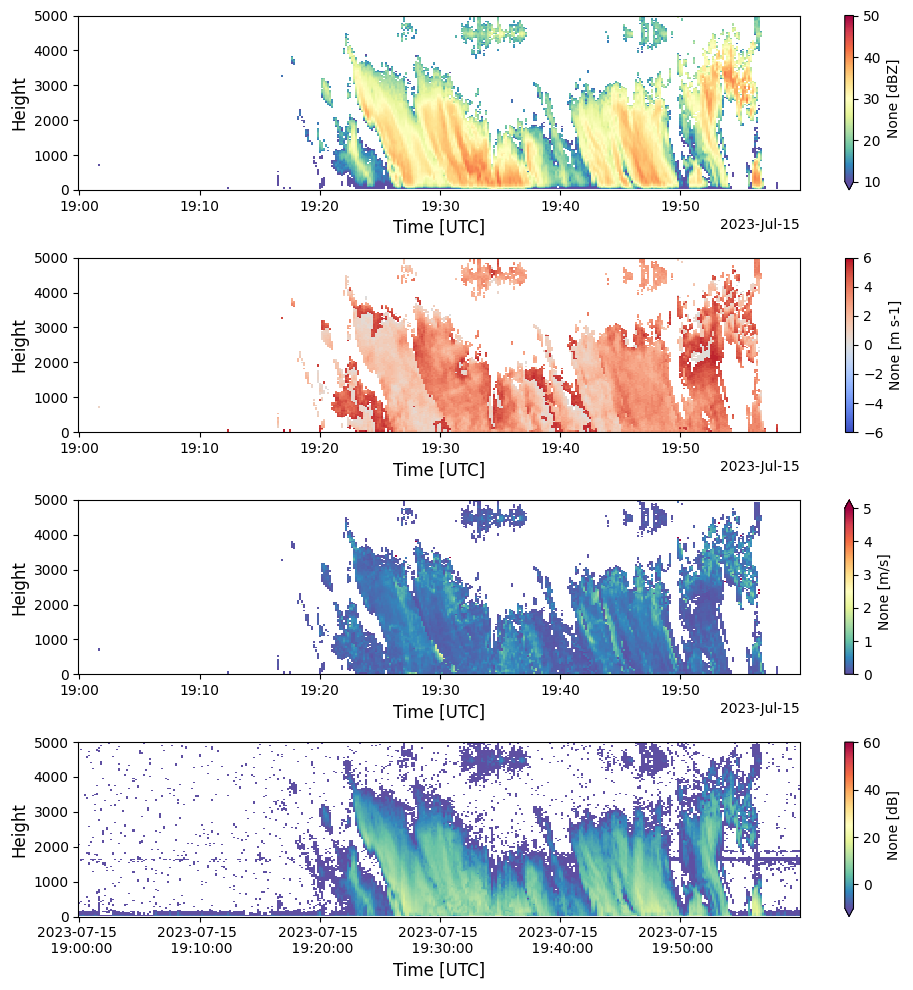
Let’s show 4 plots in one, just in case you want to see how different variables interact. This is a graph of Attenuation Corrected Reflectivity, Doppler Velocity, Spectral Width, and Signal to Noise Ratio vs. Height.

fig, ax = plt.subplots(4, 1, figsize=(10, 10))
ds["Zea"].T.plot(cmap='Spectral_r', vmin=10, vmax=50, ax=ax[0])
ax[0].set_xlabel('Time [UTC]', fontsize=12), ax[0].set_ylabel('Height', fontsize=12)
ax[0].set_ylim(0, 5000)
ds["VEL"].T.plot(cmap='coolwarm', vmin=-6, vmax=6, ax=ax[1])
ax[1].set_xlabel('Time [UTC]', fontsize=12), ax[1].set_ylabel('Height', fontsize=12)
ax[1].set_ylim(0, 5000)
ds["WIDTH"].T.plot(cmap='Spectral_r', vmin=0, vmax=5, ax=ax[2])
ax[2].set_xlabel('Time [UTC]', fontsize=12), ax[2].set_ylabel('Height', fontsize=12)
ax[2].set_ylim(0, 5000)
ds["SNR"].T.plot(cmap='Spectral_r', vmin=-10, vmax=60, ax=ax[3])
ax[3].set_xlabel('Time [UTC]', fontsize=12), ax[3].set_ylabel('Height', fontsize=12)
ax[3].set_ylim(0, 5000)
date_form = DateFormatter("%Y-%m-%d \n %H:%M:%S")
plt.gca().xaxis.set_major_formatter(date_form)
fig.tight_layout()

../../_images/562fd462efb8b892f0938bde5c64ca60a18e7b3a9a4ceea093d44ddc89f6ced8.png

Plotting multiple hours in one plot#

The code cell below picks multiple hours in a single day, in this case 9 hours, and removes empty datasets so it creates a better plot overall.

# list comprehension for files only doing 9 files for now
dsets = [catch_bad_file(cds)
         for cds in cat.datasets[289:298]]
ds_non_none = [x for x in dsets if x is not None]
ds = xr.combine_by_coords(ds_non_none, combine_attrs='override')

Exception:  <class 'requests.exceptions.HTTPError'>

This shows the times that are being plotted and its attributes.

ds['Ze']

<xarray.DataArray 'Ze' (time: 2880, range: 256)>
array([[nan, nan, nan, ..., nan, nan, nan],
       [nan, nan, nan, ..., nan, nan, nan],
       [nan, nan, nan, ..., nan, nan, nan],
       ...,
       [nan, nan, nan, ..., nan, nan, nan],
       [nan, nan, nan, ..., nan, nan, nan],
       [nan, nan, nan, ..., nan, nan, nan]])
Coordinates:
  * range      (range) float32 0.0 35.0 70.0 ... 8.855e+03 8.89e+03 8.925e+03
  * time       (time) datetime64[ns] 2023-07-15T02:00:00.006705920 ... 2023-0...
    elevation  (time) float32 90.0 90.0 90.0 90.0 90.0 ... 90.0 90.0 90.0 90.0
    azimuth    (time) float32 0.0 0.0 0.0 0.0 0.0 0.0 ... 0.0 0.0 0.0 0.0 0.0
Attributes:
    standard_name:     equivalent_reflectivity_factor
    long_name:         None
    units:             dBZ
    field_folds:       false
    fold_limit_lower:  0.0
    fold_limit_upper:  0.0
    thresholding_xml:  None
    legend_xml:        None
    is_discreet:       false
    _ChunkSizes:       [  1 256]

xarray.DataArray

'Ze'

time: 2880
range: 256

nan nan nan nan nan nan nan nan ... nan nan nan nan nan nan nan nan

array([[nan, nan, nan, ..., nan, nan, nan],
       [nan, nan, nan, ..., nan, nan, nan],
       [nan, nan, nan, ..., nan, nan, nan],
       ...,
       [nan, nan, nan, ..., nan, nan, nan],
       [nan, nan, nan, ..., nan, nan, nan],
       [nan, nan, nan, ..., nan, nan, nan]])

Coordinates: (4)
- range
  (range)
  float32
  0.0 35.0 ... 8.89e+03 8.925e+03
  standard_name :
  projection_range_coordinate
  long_name :
  range_to_measurement_volume
  units :
  meters
  spacing_is_constant :
  true
  meters_to_center_of_first_gate :
  0.0
  meters_between_gates :
  35.0
  axis :
  radial_range_coordinate
```
array([   0.,   35.,   70., ..., 8855., 8890., 8925.], dtype=float32)
```
- time
  (time)
  datetime64[ns]
  2023-07-15T02:00:00.006705920 .....
  long_name :
  time_in_seconds_since_volume_start
  standard_name :
  time
  _ChunkSizes :
  512
```
array(['2023-07-15T02:00:00.006705920', '2023-07-15T02:00:10.006702848',
       '2023-07-15T02:00:20.006696960', ..., '2023-07-15T19:59:30.006707968',
       '2023-07-15T19:59:40.006707968', '2023-07-15T19:59:50.006724096'],
      dtype='datetime64[ns]')
```
- elevation
  (time)
  float32
  90.0 90.0 90.0 ... 90.0 90.0 90.0
  standard_name :
  ray_elevation_angle
  long_name :
  elevation_angle_from_horizontal_plane
  units :
  degrees
  axis :
  radial_elevation_coordinate
  _ChunkSizes :
  1024
```
array([90., 90., 90., ..., 90., 90., 90.], dtype=float32)
```
- azimuth
  (time)
  float32
  0.0 0.0 0.0 0.0 ... 0.0 0.0 0.0 0.0
  standard_name :
  ray_azimuth_angle
  long_name :
  azimuth_angle_from_true_north
  units :
  degrees
  axis :
  radial_azimuth_coordinate
  _ChunkSizes :
  1024
```
array([0., 0., 0., ..., 0., 0., 0.], dtype=float32)
```

Indexes: (2)

range

PandasIndex

PandasIndex(Float64Index([   0.0,   35.0,   70.0,  105.0,  140.0,  175.0,  210.0,  245.0,
               280.0,  315.0,
              ...
              8610.0, 8645.0, 8680.0, 8715.0, 8750.0, 8785.0, 8820.0, 8855.0,
              8890.0, 8925.0],
             dtype='float64', name='range', length=256))

time

PandasIndex

PandasIndex(DatetimeIndex(['2023-07-15 02:00:00.006705920',
               '2023-07-15 02:00:10.006702848',
               '2023-07-15 02:00:20.006696960',
               '2023-07-15 02:00:30.006696960',
               '2023-07-15 02:00:40.006712832',
               '2023-07-15 02:00:50.006719232',
               '2023-07-15 02:01:00.006701824',
               '2023-07-15 02:01:10.006697984',
               '2023-07-15 02:01:20.006705920',
               '2023-07-15 02:01:30.006701824',
               ...
               '2023-07-15 19:58:20.006721024',
               '2023-07-15 19:58:30.006700032',
               '2023-07-15 19:58:40.006722816',
               '2023-07-15 19:58:50.006722048',
               '2023-07-15 19:59:00.006691072',
               '2023-07-15 19:59:10.006705152',
               '2023-07-15 19:59:20.006705152',
               '2023-07-15 19:59:30.006707968',
               '2023-07-15 19:59:40.006707968',
               '2023-07-15 19:59:50.006724096'],
              dtype='datetime64[ns]', name='time', length=2880, freq=None))

Attributes: (10)
standard_name :
equivalent_reflectivity_factor
long_name :
None
units :
dBZ
field_folds :
false
fold_limit_lower :
0.0
fold_limit_upper :
0.0
thresholding_xml :
None
legend_xml :
None
is_discreet :
false
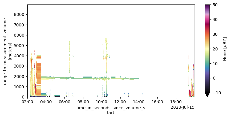
_ChunkSizes :
[ 1 256]

A plot of equivalent reflectivity for the hours of July 15th, 2023. As you notice there is rain at 19:00

plt.figure(figsize=(9, 4))
ds['Ze'].plot(x='time', cmap='ChaseSpectral', vmin=-10, vmax=50)
#plt.savefig('July 15.png', dpi=300, bbox_inches='tight')

<matplotlib.collections.QuadMesh at 0x14cf14730>

../../_images/2b4e3df361922e5481fb50cec9c407b8f5e33d9ad57613b562df85d3cb1217ff.png

Summary#

Within this notebook, we covered the basics of working with MRR radar data using the CROCUS Thredds Server, including:

Reading the MRR data through the CROCUS Thredds Server
Visualizing the radar data

Resources and References#

CROCUS Thredds Server essential link:

Thredds

Loading And Visualizing mrr datA (LAVA)

Contents

Loading And Visualizing mrr datA (LAVA)#

Overview#

Prerequisites#

Installation#

An Overview of the MRR-Pro#

Imports#

Data Preprocessing#

Accessing the CROCUS Thredds server#

Testing the code#

Sample plot using the test data#

Visualizing the MRR data#

Plotting one hour in a single plot#

Plotting multiple hours in one plot#

Summary#

Resources and References#